The End of Growth in 2019?

2019: World Economy Is Reaching Growth Limits; Expect Low Oil Prices, Financial Turbulence

Zero Hedge,

12 January, 2019

Authored by Gail Tverberg via Our Finite World blog,

Financial markets have been behaving in a very turbulent manner in the last couple of months. The issue, as I see it, is that the world economy is gradually shifting from a growth mode to a mode of shrinkage. This is something like a ship changing course, from going in one direction to going in reverse. The system acts as if the brakes are being very forcefully applied, and reaction of the economy is to almost shake.

What seems to be happening is that the world economy is reaching Limits to Growth, as predicted in the computer simulations modeled in the 1972 book, The Limits to Growth. In fact, the base model of that set of simulations indicated that peak industrial output per capita might be reached right about now. Peak food per capita might be reached about the same time. I have added a dotted line to the forecast from this model, indicating where the economy seems to be in 2019, relative to the base model.

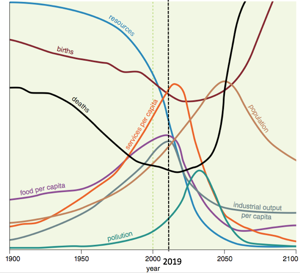
Figure 1. Base scenario from The Limits to Growth, printed using today’s graphics by Charles Hall and John Day in Revisiting Limits to Growth After Peak Oil with dotted line at 2019 added by author. The 2019 line is drawn based on where the world economy seems to be now, rather than on precisely where the base model would put the year 2019.

The economy is a self-organizing structure that operates under the laws of physics. Many people have thought that when the world economy reaches limits, the limits would be of the form of high prices and “running out” of oil. This represents an overly simple understanding of how the system works. What we should really expect, and in fact, what we are now beginning to see, is production cuts in finished goods made by the industrial system, such as cell phones and automobiles, because of affordability issues. Indirectly, these affordability issues lead to low commodity prices and low profitability for commodity producers. For example:

• The sale of Chinese private passenger vehicles for the year of 2018 through November is down by 2.8%, with November sales off by 16.1%. Most analysts are forecasting this trend of contracting sales to continue into 2019. Lower sales seem to reflect affordability issues.
• Saudi Arabia plans to cut oil production by 800,000 barrels per day from the November 2018 level, to try to raise oil prices. Profits are too low at current prices.
• Coal is reported not to have an economic future in Australia, partly because of competition from subsidized renewables and partly because China and India want to prop up the prices of coal from their own coal mines.

The Significance of Trump’s Tariffs

If a person looks at history, it becomes clear that tariffs are a standard response to a problem of shrinking food or industrial output per capita. Tariffs were put in place in the 1920s in the time leading up to the Great Depression, and were investigated after the Panic of 1857, which seems to have indirectly led to the US Civil War.

Whenever an economy produces less industrial or food output per capita there is an allocation problem: who gets cut off from buying output similar to the amount that they previously purchased? Tariffs are a standard way that a relatively strong economy tries to gain an advantage over weaker economies. Tariffs are intended to help the citizens of the strong economy maintain their previous quantity of goods and services, even as other economies are forced to get along with less.

I see Trump’s trade policies primarily as evidence of an underlying problem, namely, the falling affordability of goods and services for a major segment of the population. Thus, Trump’s tariffs are one of the pieces of evidence that lead me to believe that the world economy is reaching Limits to Growth.

The Nature of World Economic Growth

Economic growth seems to require growth in three dimensions (a) Complexity, (b) Debt Bubble, and (c) Use of Resources. Today, the world economy seems to be reaching limits in all three of these dimensions (Figure 2).

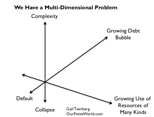
Figure 2.

Complexity involves adding more technology, more international trade and more specialization. Its downside is that it indirectly tends to reduce affordability of finished end products because of growing wage disparity; many non-elite workers have wages that are too low to afford very much of the output of the economy. As more complexity is added, wage disparity tends to increase. International wage competition makes the situation worse.

A growing debt bubble can help keep commodity prices up because a rising amount of debt can indirectly provide more demand for goods and services. For example, if there is growing debt, it can be used to buy homes, cars, and vacation travel, all of which require oil and other energy consumption.

If debt levels become too high, or if regulators decide to raise short-term interest rates as a method of slowing the economy, the debt bubble is in danger of collapsing. A collapsing debt bubble tends to lead to recession and falling commodity prices. Commodity prices fell dramatically in the second half of 2008. Prices now seem to be headed downward again, starting in October 2018.

Figure 3. Brent oil prices with what appear to be debt bubble collapses marked.

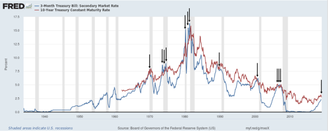
Figure 4. Three-month treasury secondary market rates compared to 10-year treasuries from FRED, with points where short term interest rates exceed long term rates marked by author with arrows.

Even the relatively slow recent rise in short-term interest rates (Figure 4) seems to be producing a decrease in oil prices (Figure 3) in a way that a person might expect from a debt bubble collapse. The sale of US Quantitative Easing assets at the same time that interest rates have been rising no doubt adds to the problem of falling oil prices and volatile stock markets. The gray bars in Figure 4 indicate recessions.

Growing use of resources becomes increasingly problematic for two reasons. One is population growth. As population rises, the economy needs more food to feed the growing population. This leads to the need for more complexity (irrigation, better seed, fertilizer, world trade) to feed the growing world population.

The other problem with growing use of resources is diminishing returns, leading to the rising cost of extracting commodities over time. Diminishing returns occur because producers tend to extract the cheapest to extract commodities first, leaving in place the commodities requiring deeper wells or more processing. Even water has this difficulty. At times, desalination, at very high cost, is needed to obtain sufficient fresh water for a growing population.

Why Inadequate Energy Supplies Lead to Low Oil Prices Rather than High

In the last section, I discussed the cost of producing commodities of many kinds rising because of diminishing returns. Higher costs should lead to higher prices, shouldn’t they?

Strangely enough, higher costs translate to higher prices only sometimes. When energy consumption per capita is rising rapidly (peaks of red areas on Figure 5), rising costs do seem to translate to rising prices. Spiking oil prices were experienced several times: 1917 to 1920; 1974 to 1982; 2004 to mid 2008; and 2011 to 2014. All of these high oil prices occurred toward the end of the red peaks on Figure 5. In fact, these high oil prices (as well as other high commodity prices that tend to rise at the same time as oil prices) are likely what brought growth in energy consumption down. The prices of goods and services made with these commodities became unaffordable for lower-wage workers, indirectly decreasing the growth rate in energy products consumed.

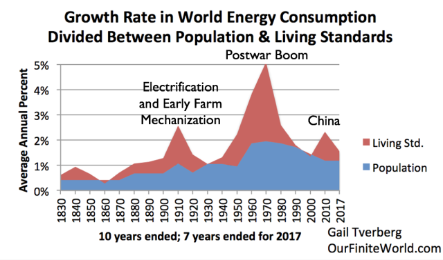
Figure 5.

The red peaks represented periods of very rapid growth, fed by growing supplies of very cheap energy: coal and hydroelectricity in the Electrification and Early Mechanizationperiod, oil in the Postwar Boom, and coal in the China period. With low energy prices,  many countries were able to expand their economies simultaneously, keeping demand high. The Postwar Boom also reflected the addition of many women to the labor force, increasing the ability of families to afford second cars and nicer homes.

Rapidly growing energy consumption allowed per capita output of both food (with meat protein given a higher count than carbohydrates) and industrial products to grow rapidly during these peaks. The reason that output of these products could grow is because the laws of physics require energy consumption for heat, transportation, refrigeration and other processes required by industrialization and farming. In these boom periods, higher energy costs were easy to pass on. Eventually the higher energy costs “caught up with” the economy, and pushed growth in energy consumption per capita down, putting an end to the peaks.

Figure 6 shows Figure 5 with the valleys labeled, instead of the peaks.

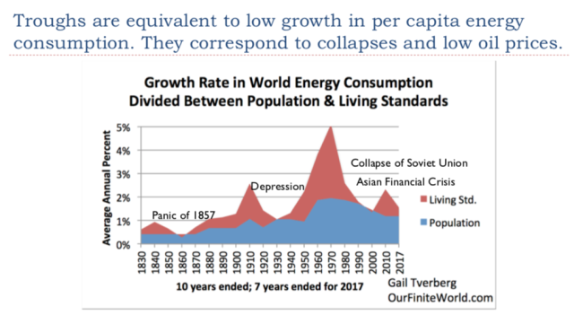
Figure 6.

When I say that the world economy is reaching “peak industrial output per capita” and “peak food per capita,” this represents the opposite of a rapidly growing economy. In fact, if the world is reaching Limits to Growth, the situation is even worse than all of the labeled valleys on Figure 6. In such a case, energy consumption growth is likely to shrink so low that even the blue area (population growth) turns negative.

In such a situation, the big problem is “not enough to go around.” While cost increases due to diminishing returns could easily be passed along when growth in industrial and food output per capita were rapidly rising (the Figure 5 situation), this ability seems to disappear when the economy is near limits. Part of the problem is that the lower growth in per capita energy affects the kinds of job that are available. With low energy consumption growth, many of the jobs that are available are service jobs that do not pay well. Wage disparity becomes an increasing problem.

When wage disparity grows, the share of low wage workers rises. If businesses try to pass along their higher costs of production, they encounter market resistance because lower wage workers cannot afford the finished goods made with high cost energy products. For example, auto and iPhone sales in China decline. The lack of Chinese demand tends to lead to a drop in demand for the many commodities used in manufacturing these goods, including both energy products and metals. Because there is very little storage capacity for commodities, a small decline in demand tends to lead to quite a large decline in prices. Even a small decline in China’s demand for energy products can lead to a big decline in oil prices.

Strange as it may seem, the economy ends up with low oil prices, rather than high oil prices, being the problem. Other commodity prices tend to be low as well.

What Is Ahead, If We Are Reaching Economic Growth Limits?

1. Figure 1 at the top of this post seems to give an indication of what is ahead after 2019, but this forecast cannot be relied on. A major issue is that the limited model used at that time did not include the financial system or debt. Even if the model seems to provide a reasonably accurate estimate of when limits will hit, it won’t necessarily give a correct view of what the impact of limits will be on the rest of the economy, after limits hit. The authors, in fact, have said that the model should not be expected to provide reliable indications regarding how the economy will behave after limits have started to have an impact on economic output.

2. As indicated in the title of this post, considerable financial volatility can be expected in 2019 if the economy is trying to slow itself. Stock prices will be erratic; interest rates will be erratic; currency relativities will tend to bounce around. The likelihood that derivatives will cause major problems for banks will rise because derivatives tend to assume more stability in values than now seems to be the case. Increasing problems with derivatives raises the risk of bank failure.

3. The world economy doesn’t necessarily fail all at once. Instead, pieces that are, in some sense, “less efficient” users of energy may shrink back. During the Great Recession of 2008-2009, the countries that seemed to be most affected were countries such as Greece, Spain, and Italy that depend on oil for a disproportionately large share of their total energy consumption. China and India, with energy mixes dominated by coal, were much less affected.

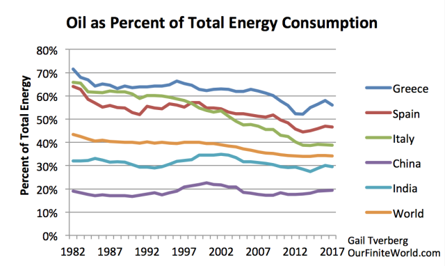
Figure 7. Oil consumption as a percentage of total energy consumption, based on 2018 BP Statistical Review of World Energy data.

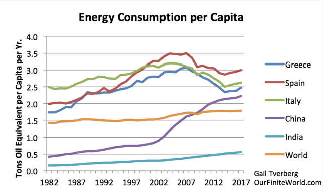
Figure 8. Energy consumption per capita for selected areas, based on energy consumption data from 2018 BP Statistical Review of World Energy and United Nations 2017 Population Estimates by Country.

In the 2002-2008 period, oil prices were rising faster than prices of other fossil fuels. This tended to make countries using a high share of oil in their energy mix less competitive in the world market. The low labor costs of China and India gave these countries another advantage. By the end of 2007, China’s energy consumption per capita had risen to a point where it almost matched the (now lower) energy consumption of the European countries shown. China, with its low energy costs, seems to have “eaten the lunch” of some of its European competitors.

In 2019 and the years that follow, some countries may fare at least somewhat better than others. The United States, for now, seems to be faring better than many other parts of the world.

4. While we have been depending upon China to be a leader in economic growth, China’s growth is already faltering and may turn to contraction in the near future. One reason is an energy problem: China’s coal production has fallen because many of its coal mines have been closed due to lack of profitability. As a result, China’s need for imported energy (difference between black line and top of energy production stack) has been growing rapidly. China is now the largest importer of oil, coal, and natural gas in the world. It is very vulnerable to tariffs and to lack of available supplies for import.

Figure 9. China energy production by fuel plus its total energy consumption, based on BP Statistical Review of World Energy 2018 data.

A second issue is that demographics are working against China; its working-age population already seems to be shrinking. A third reason why China is vulnerable to economic difficulties is because of its growing debt level. Debt becomes difficult to repay with interest if the economy slows.

5. Oil exporters such as Venezuela, Saudi Arabia, and Nigeria have become vulnerable to government overthrow or collapse because of low world oil prices since 2014. If the central government of one or more of these exporters disappears, it is possible that the pieces of the country will struggle along, producing a lower amount of oil, as Libya has done in recent years. It is also possible that another larger country will attempt to take over the failing production of the country and secure the output for itself.

6. Epidemics become increasingly likely, especially in countries with serious financial problems, such as Yemen, Syria, and Venezuela. Historically, much of the decrease in population in countries with collapsing economies has come from epidemics. Of course, epidemics can spread across national boundaries, exporting the problems elsewhere.

7. Resource wars become increasingly likely. These can be local wars, perhaps over the availability of water. They can also be large, international wars. The timing of World War I and World War II make it seem likely that these wars were both resource wars.

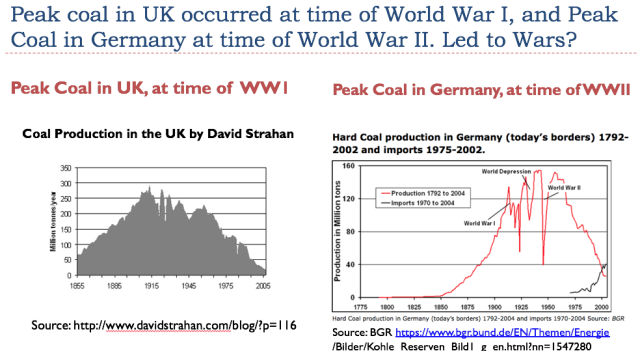
Figure 10.

8. Collapsing intergovernmental agencies, such as the European Union, the World Trade Organization, and the International Monetary Fund, seem likely. The United Kingdom’s planned exit from the European Union in 2019 is a step toward dissolving the European Union.

9. Privately funded pension funds will increasingly be subject to default because of continued low interest rates. Some governments may choose to cut back the amounts they provide to pensioners because governments cannot collect adequate tax revenue for this purpose. Some countries may purposely shut down parts of their governments, in an attempt to hold down government spending.

10. A far worse and more permanent recession than that of the Great Recession seems likely because of the difficulty in repaying debt with interest in a shrinking economy. It is not clear when such a recession will start. It could start later in 2019, or perhaps it may wait until 2020. As with the Great Recession, some countries will be affected more than others. Eventually, because of the interconnected nature of financial systems, all countries are likely to be drawn in.

Summary

It is not entirely clear exactly what is ahead if we are reaching Limits to Growth. Perhaps that is for the best. If we cannot do anything about it, worrying about the many details of what is ahead is not the best for anyone’s mental health. While it is possible that this is an end point for the human race, this is not certain, by any means. There have been many amazing coincidences over the past 4 billion years that have allowed life to continue to evolve on this planet. More of these coincidences may be ahead. We also know that humans lived through past ice ages. They likely can live through other kinds of adversity, including worldwide economic collapse.

The Great Depression was an energy crisis - Gail Tverberg

The Depression Of The 1930s Was An Energy Crisis

Zero Hedge,

19 December, 2017

Authored by Gail Tverberg via Our Finite World blog,

Economists, including Ben Bernanke, give all kinds of reasons for the Great Depression of the 1930s. But what if the real reason for the Great Depression was an energy crisis?

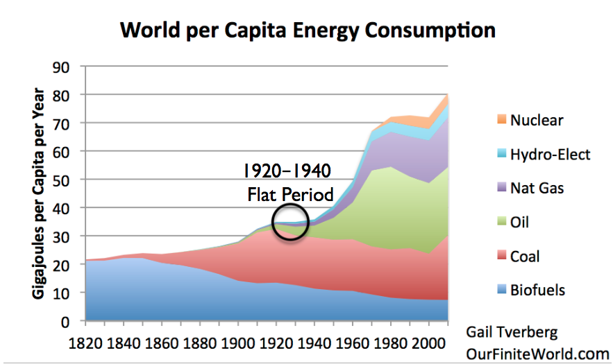
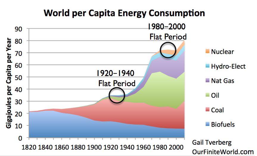
When I put together a chart of per capita energy consumption since 1820 for a post back in 2012, there was a strange “flat spot” in the period between 1920 and 1940. When we look at the underlying data, we see that coal production was starting to decline in some of the major coal producing parts of the world at that time. From the point of view of people living at the time, the situation might have looked very much like peak energy consumption, at least on a per capita basis.

Figure 1. World Energy Consumption by Source, based on Vaclav Smil estimates from Energy Transitions: History, Requirements and Prospects (Appendix) together with BP Statistical Data for 1965 and subsequent, divided by population estimates by Angus Maddison.

Even back in the 1820 to 1900 period, world per capita energy had gradually risen as an increasing amount of coal was used. We know that going back a very long time, the use of water and wind had never amounted to very much (Figure 2) compared to burned biomass and coal, in terms of energy produced. Humans and draft animals were also relatively low in energy production. Because of its great heat-producing ability, coal quickly became the dominant fuel.

Figure 2. Annual energy consumption per head (megajoules) in England and Wales during the period 1561-70 to 1850-9 and in Italy from 1861-70. Figure by Wrigley

In general, we know that energy products, including coal, are necessary to enable processes that contribute to economic growth.Heat is needed for almost all industrial processes. Transportation needs energy products of one kind or another. Building roads and homes requires energy products. It is not surprising that the Industrial Revolution began in Britain, with its use of coal.

We also know that there is a long-term correlation between world GDP growth and energy consumption.

Figure 3. X-Y graph of world energy consumption (from BP Statistical Review of World Energy, 2017) versus world GDP in 2010 US$, from World Bank.

The “flat period” in 1920-1940 in Figure 1 was likely problematic. The economy is a self-organized networked system; what was wrong could be expected to appear in many parts of the economy. Economic growth was likely far too low. The chance for conflict among nations was much higher because of stresses in the system–there was not really enough coal to go around. These stresses could extend to the period immediately before 1920 and after 1940, as well.

A Peak in Coal Production Hit UK, United States, and Germany at Close to the Same Time

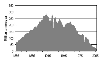
This is a coal supply chart for UK. Its peak coal production (which was an all time peak) was in 1913. The UK was the largest coal producer in Europe at the time.

Figure 3. United Kingdom coal production since 1855, in figure by David Strahan. First published in New Scientist, 17 January 2008.

The United States hit a peak in its production only five years later, in 1918. This peak was only a “local” peak. There were also later peaks, in 1947 and 2008, after coal production was developed in new areas of the country.

Figure 4. US coal production, in Wikipedia exhibit by contributor Plazak.

By type, US coal production is as shown on Figure 5.

Figure 5. US coal production by type, in Wikipedia exhibit by contributor Plaza.

Evidently, the highest quality coal, Anthracite, reached a peak and began to decline about 1918. Bituminous coal hit a peak about the same time, and dropped way back in production during the 1930s. The poorer quality coals were added later, as the better-quality coals became less abundant.

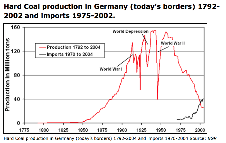
The pattern for Germany’s hard coal shows a pattern somewhat in between the UK and the US pattern.

Figure 6. Source GBR.

Germany too had a peak during World War I, then dropped back for several years. It then had three later peaks, the highest one during World War II.

What Affects Coal Production?

If there is a shortage of coal, fixing it is not as simple as “inadequate coal supply leads to higher price,” quickly followed by “higher price leads to more production.” Clearly the amount of coal resource in the ground affects the amount of coal extraction, but other things do as well.

[1] The amount of built infrastructure for taking the coal out and delivering the coal. Usually, a country only adds a little coal extraction capacity at a time and leaves the rest in the ground. (This is how the US and Germany could have temporary coal peaks, which were later surpassed by higher peaks.) To add more extraction capacity, it is necessary to add (a) investment needed for getting the coal out of the ground as well as (b) infrastructure for delivering coal to potential users. This includes things like trains and tracks, and export terminals for coal transported by boats.

[2] Prices available in the marketplace for coal. These fluctuate widely. We will discuss this more in a later section. Clearly, the higher the price, the greater the quantity of coal that can be extracted and delivered to users.

[3] The cost of extraction, both in existing locations and in new locations. These costs can perhaps be reduced if it is possible to add new technology. At the same time, there is a tendency for costs within a given mine to increase over time, as it becomes necessary to access deeper, thinner seams. Also, mines tend to be built in the most convenient locations first, with best access to transportation. New mines very often will be higher cost, when these factors are considered.

[4] The cost and availability of capital (shares of stock and sale of debt) needed for building new infrastructure, and for building new devices made possible by new technology. These are affected by interest rates and tax levels.

[5] Time lags needed to implement changes. New infrastructure and new technology are likely to take several years to implement.

[6] The extent to which wages can be recycled into demand for energy products. An economy needs to have buyers for the products it makes. If a large share of the workers in an economy is very low-paid, this creates a problem.

If there is an energy shortage, many people think of the shortage as causing high prices. In fact, the shortage is at least equally likely to cause greater wage disparity. This might also be considered a shortage of jobs that pay well. 

Without jobs that pay well, would-be workers find it hard to purchase the many goods and services created by the economy (such as homes, cars, food, clothing, and advanced education). For example, young adults may live with their parents longer, and elderly people may move in with their children.

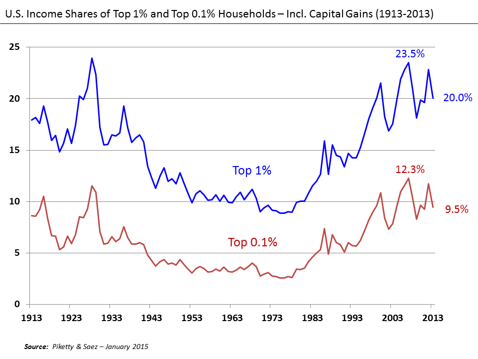
The lack of jobs that pay well tends to hold down “demand” for goods made with commodities, and thus tends to bring down commodity prices. This problem happened in the 1930s and is happening again today. The problem is an affordability problem, but it is sometimes referred to as “low demand.” Workers with inadequate wages cannot afford to buy the goods made by the economy. There may be a glut of a commodity (food, or oil, or coal), and commodity prices that fall far below what producers need to make a profit.

Figure 7. U. S. Income Shares of Top 10% and Top 1%, Wikipedia exhibit by Piketty and Saez.

The Fluctuating Nature of Commodity Prices

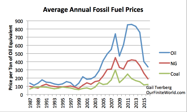
I have noted in the past that fossil fuel prices tend to move together. This is what we would expect, if affordability is a major issue, and affordability changes over time.

Figure 8. Price per ton of oil equivalent, based on comparative prices for oil, natural gas, and coal given in BP Statistical Review of World Energy. Not inflation adjusted.

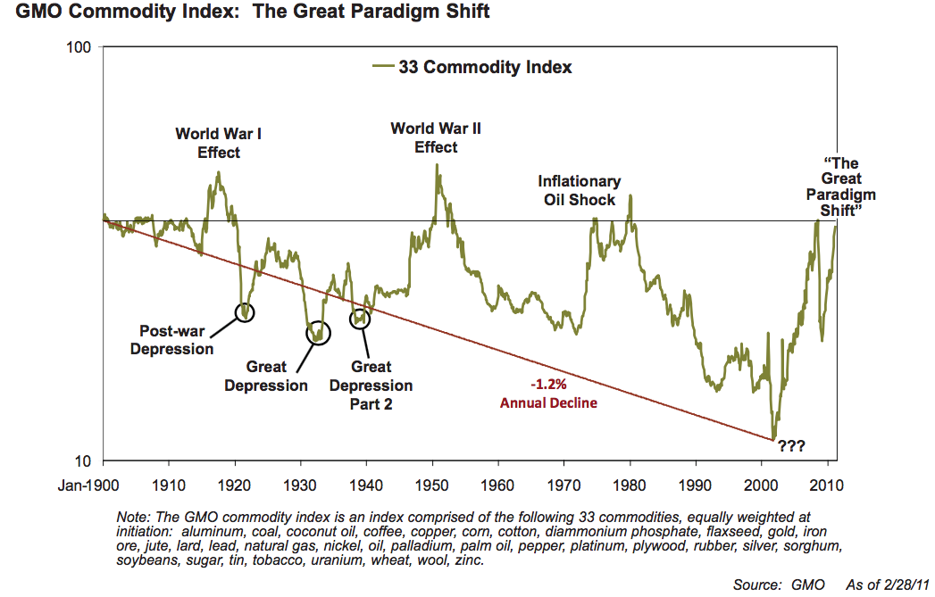
We would expect metal prices to follow fossil fuel prices, because fossil fuels are used in the extraction of ores of all kinds. Investment strategist Jeremy Grantham (and his company GMO) noted this correlation among commodity prices, and put together an index of commodity prices back to 1900.

Figure 9. GMO Commodity Index 1900 to 2011, from GMO April 2011 Quarterly Letter. “The Great Paradigm Shift,” shown at the end is not really the correct explanation, something now admitted by Grantham. If the graph were extended beyond 2010, it would show high prices in 2010 to 2013. Prices would fall to a much lower level in 2014 to 2017.

Reason for the Spikes in Prices. As we will see in the next few paragraphs, the spikes in prices generally arise in situations in which everyday goods (food, homes, clothing, transportation) suddenly became more affordable to “non-elite” workers. These are workers who are not highly educated, and are not in supervisory positions. These spikes in prices don’t generally “come about” by themselves; instead, they are engineered by governments, trying to stimulate the economy.

In both the World War I and World War II price spikes, governments greatly raised their debt levels to fund the war efforts. Some of this debt likely went directly into demand for commodities, such as to make more bombs, and to operate tanks, and thus tended to raise commodity prices. In addition, quite a bit of the debt indirectly led to more employment during the period of the war. For example, women who were not in the workforce were hired to take jobs that had been previously handled by men who were now part of the war effort. (These women were new non-elite workers.) Their earnings helped raise demand for goods and services of all kinds, and thus commodity prices.

The 2008 price spike was caused (at least in part) by a US housing-related debt bubble. Interest rates were lowered in the early 2000s to stimulate the economy. Also, banks were encouraged to lend to people who did not seem to meet usual underwriting standards. The additional demand for houses raised prices. Homeowners, wishing to cash in on the new higher prices for their homes, could refinance their loans and withdraw the cash related to the new higher prices. They could use the funds withdrawn to buy goods such as a new car or a remodeled basement. These withdrawn funds indirectly supplemented the earnings of non-elite workers (as did the lower interest rate on new borrowing).

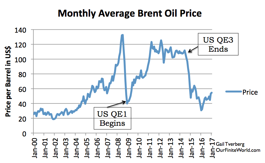
The 2011-2014 spike was caused by the extremely low interest rates made possible by Quantitative Easing. These low interest rates made the buying of homes and cars more affordable to all buyers, including non-elite workers. When the US discontinued its QE program in 2014, the US dollar rose relative to many other currencies, making oil and other fuels relatively more expensive to workers outside the US. These higher costs reduced the demand for fuels, and dropped fuel prices back down again.

Figure 10. Monthly Brent oil prices with dates of US beginning and ending QE.

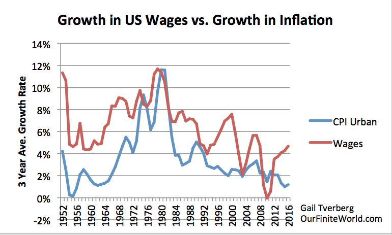
The run-up in oil prices (and other commodity prices) in the 1970s is widely attributed to US oil production peaking, but I think that the rapid run-up in prices was enabled by the rapid wage run-up of the period (Figure 11 below).

Figure 11. Growth in US wages versus increase in CPI Urban. Wages are total “Wages and Salaries” from US Bureau of Economic Analysis. CPI-Urban is from US Bureau of Labor Statistics.

The Opposing Force: Energy prices need to fall, if the economy is to grow. All of these upward swings in prices can be at most temporary changes to the long-term downward trend in prices. Let’s think about why.

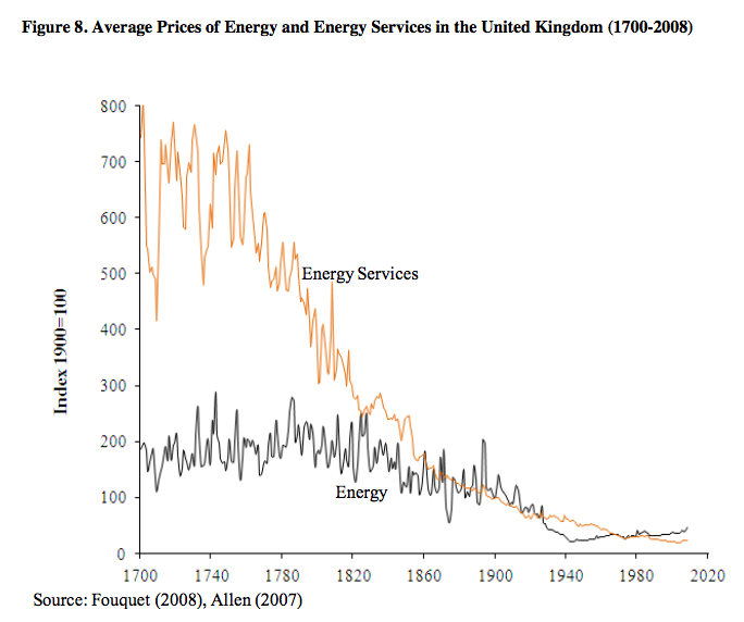
An economy needs to grow. To do so, it needs an increasing supply of commodities, particularly energy commodities. This can only happen if energy prices are trending lower. These lower prices enable the purchase of greater supply. We can see this in the results of some academic papers. For example, Roger Fouquet shows that it is not the cost of energy, per se, that drops over time. Rather, it is the cost of energy services that declines.

Figure 12. Total Cost of Energy and Energy Services, by Roger Fouquet, from Divergences in Long Run Trends in the Prices of Energy and Energy Services.

Energy services include changes in efficiency, besides energy costs themselves. 

Thus, Fouquet is looking at the cost of heating a home, or the cost of electrical services, or the cost of transportation services, in inflation-adjusted units.

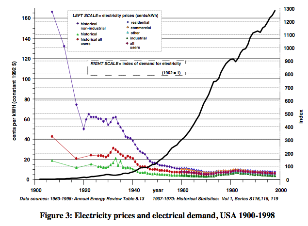
Robert Ayres and Benjamin Warr show a similar result, related to electricity. They also show that usage tends to rise, as prices fall.

Figure 13. Ayres and Warr Electricity Prices and Electricity Demand, from “Accounting for growth: the role of physical work.”

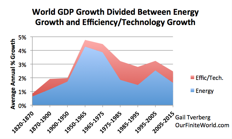
Ultimately, we know that the growth in energy consumption tends to rise at close to the same rate as the growth in GDP. To keep energy consumption rising, it is helpful if the cost of energy services is falling.

Figure 14. World GDP growth compared to world energy consumption growth for selected time periods since 1820. World real GDP trends for 1975 to present are based on USDA real GDP data in 2010$ for 1975 and subsequent. (Estimated by author for 2015.) GDP estimates for prior to 1975 are based on Maddison project updates as of 2013. Growth in the use of energy products is based on a combination of data from Appendix A data from Vaclav Smil’s Energy Transitions: History, Requirements and Prospects together with BP Statistical Review of World Energy 2015 for 1965 and subsequent.

How the Economic Growth Pump Works

There seems to be a widespread belief, “We pay each other’s wages.” If this is all that there is to economic growth, all that is needed to make the economy grow faster is for each of us to sell more services to each other (cut each other’s hair more often, or give each other back rubs, and charge for them ). I think this story is very incomplete.

The real story is that energy products can be used to leverage human labor. For example, it is inefficient for a human to walk to deliver goods to customers. If a human can drive a truck instead, it leverages his ability to deliver goods. The more leveraging that is available for human labor, the more goods and services that can be produced in total, and the higher inflation-adjusted wages can be. This increased leveraging of human labor allows inflation-adjusted wages to rise. Some might call this result, “a higher return on human labor.”

These higher wages need to go back to the non-elite workers, in order to keep the growth-pump operating. With higher-wages, these workers can afford to buy goods and services made with commodities, such as homes, cars, and food.

 They can also heat their homes and operate their vehicles. These wages help maintain the demand needed to keep commodity prices high enough to encourage more commodity production.

Raising wages for elite workers (such as managers and those with advanced education), or paying more in dividends to shareholders, doesn’t have the same effect. These individuals likely already have enough money to buy the necessities of life. They may use the extra income to buy shares of stock or bonds to save for retirement, or they may buy services (such as investment advice) that require little use of energy.

The belief, “We pay each other’s wages,” becomes increasingly false, if wages and wealth are concentrated in the hands of relatively few. For example, poor people become unable to afford doctors’ visits, even with insurance, if wage disparity becomes too great. It is only when wages are fairly equal that all can afford a wide range of services provided by others in the economy.

What Went Wrong in 1920 to 1940?

Very clearly, the first thing that went wrong was the peaking of UK coal production in 1913. Even before 1913, there were pressures coming from the higher cost of coal production, as mines became more depleted. In 1912, there was a 37-day national coal strike protesting the low wages of workers. Evidently, as extraction was becoming more difficult, coal prices were not able to rise sufficiently to cover all costs, and miners’ wages were suffering. The debt for World War I seems to have helped raise commodity prices to allow wages to be somewhat higher, even if coal production did not return to its previous level.

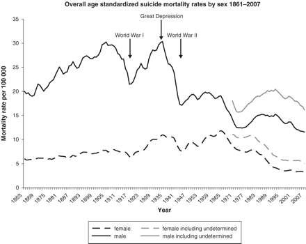
Suicide rates seem to behave inversely compared to earning power of non-elite workers. A study of suicide rates in England and Walesshows that these were increasing prior to World War I. This is what we would expect, if coal was becoming increasingly difficult to extract, and because of this, the returns for everyone, from owners to workers, was low.

Figure 15. Suicide rates in England and Wales 1861-2007 by Kyla Thomas and David Gunnell from International Journal of Epidemiology, 2010.

World War I, with its increased debt (which was in part used for more wages), helped the situation temporarily. But after World War I, the Great Depression set in, and with it, much higher suicide rates.

The Great Depression is the kind of result we would expect if UK no longer had enough coal to make the goods and services it had made previously. The lower production of goods and services would likely be paired with fewer jobs that paid well. In such a situation, it is not surprising that suicide rates rose. Suicide rates decreased greatly with World War II, and with all of the associated borrowing.

Looking more at what happened in the 1920 to 1940 period, Ugo Bardi tells us that prior to World War I, UK exported coal to Italy. With falling coal production, UK could no longer maintain those exports after World War I. This worsened relations with Italy, because Italy needed coal imported from UK to rebuild after the war. Ultimately, Italy aligned with Germany because Germany still had coal available to export. This set up the alliance for World War II.

Looking at the US, we see that World War I caused favorable conditions for exports, because with all of the fighting, Europe needed to import more goods (including food) from the United States. After the war ended in 1918, European demand was suddenly lower, and US commodity prices fell. American farmers found their incomes squeezed. As a result, they cut back on buying goods of many kinds, hurting the US economy.

One analysis of the economy of the 1920s tells us that from 1920 to 1921, farm prices fell at a catastrophic rate. “The price of wheat, the staple crop of the Great Plains, fell by almost half. The price of cotton, still the lifeblood of the South, fell by three-quarters. Farmers, many of whom had taken out loans to increase acreage and buy efficient new agricultural machines like tractors, suddenly couldn’t make their payments.”

In 1943, M. King Hubbert offered the view that all-time employment had peaked in 1920, except to the extent that it was jacked up by unusual means, such as war. In fact, some historical data shows that for four major industries combined (foundries, meat packing, paper, and printing), the employment index rose from 100 in 1914, to 157 in 1920. By September 1921, the employment index had fallen back to 89. The peak coal problem of UK had been exported to the US as low commodity prices and low employment.

It was not until the huge amount of debt related to World War II that the world economy could be stimulated enough so that total energy production per capita could continue to rise. The use of oil especially became much greater starting after World War II. It was the availability of cheap oil that allowed the world economy to grow again.

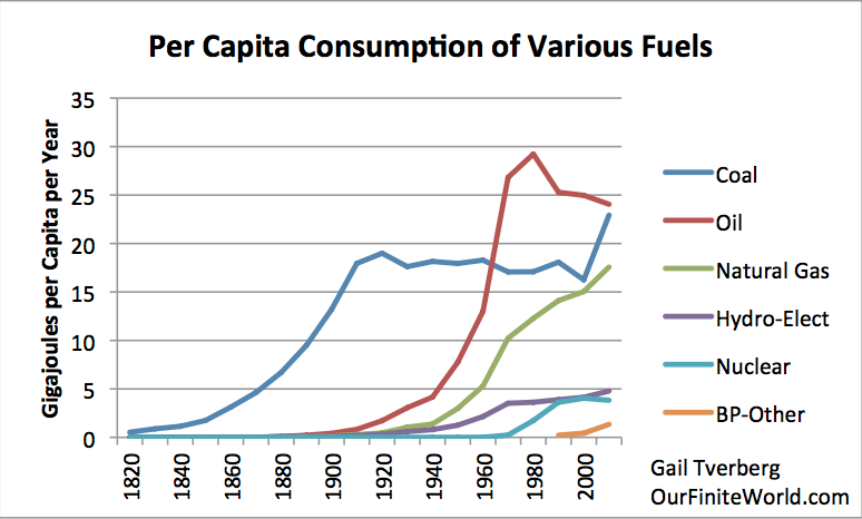
Figure 16. Per capita energy consumption by fuel, separately for several energy sources, using the same data as in Figure 1.

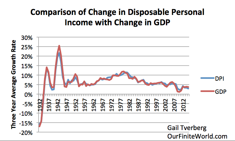
The stimulus of all the debt-enabled spending for World War II seems to have been what finally encouraged the production of the oil needed to pull the world economy out of the problems it was having. GDP and Disposable Personal Income could again rise (Figure 17.)

Figure 17. Comparison of 3-year average change in disposable personal income with 3-year change average in GDP, based on US BEA Tables 1.1.5 and 2.1.

Furthermore, total per capita energy consumption began to rise, with growing oil consumption (Figure 1). This growth in energy consumption per capita seems to be what allows the world economy to row.

I might note that there is one other exceptional period: 1980 to 2000. Space does not allow for an explanation of the situation here, but falling per capita energy consumption seems to have led to the collapse of the former Soviet Union in 1991. This was a different situation, caused by lower oil consumption related to efficiency gains. This was a situation of an oil producer being “squeezed out” because additional oil was not needed at that time. This is an example of a different type of economic disruption caused by flat per capita energy consumption.

Figure 18. World per Capita Energy Consumption with two circles relating to flat consumption. World Energy Consumption by Source, based on Vaclav Smil estimates from Energy Transitions: History, Requirements and Prospects (Appendix) together with BP Statistical Data for 1965 and subsequent, divided by population estimates by Angus Maddison.

Conclusion

There have been many views put forth about what caused the Depression of the 1930s. To my knowledge, no one has put forth the explanation that the Depression was caused by Peak Coal in 1913 in UK, and a lack of other energy supplies that were growing rapidly enough to make up for this loss. As UK “exported” this problem around the world, it led to greater wage disparity. US farmers were especially affected; their incomes often dropped below the level needed for families to buy the necessities of life.

The issue, as I have discussed in previous posts, is a physics issue. Creating GDP requires energy; when not enough energy (often fossil fuels) is available, the economy tends to “freeze out” the most vulnerable. Often, it does this by increased wage disparity. The people at the top of the hierarchy still have plenty. It is the people at the bottom who find themselves purchasing less and less. Because there are so many people at the bottom of the hierarchy, their lower purchasing power tends to pull the system down.

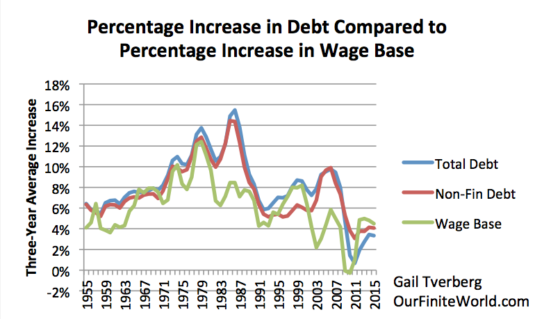
In the past, the way to get around inadequate wages for those at the bottom of the hierarchy has been to issue more debt. Some of this debt helps add more wages for non-elite workers, so helps fix the affordability problem.

Figure 19. Three-year average percent increase in debt compared to three year average percent increase in non-government wages, including proprietors’ income, which I call my wage base.

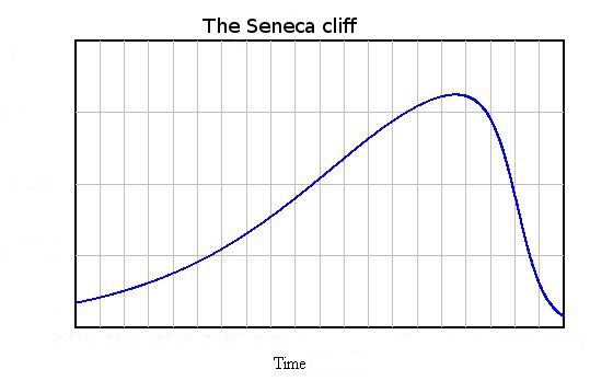
At this time, we seem to be reaching the point where, even with more debt, we are running out of cheap energy to add to the system. When this happens, the economic system seems more prone to  fracture. Ugo Bardi calls the situation “reaching the inflection point in a Seneca Cliff.”

Figure 20. Seneca Cliff by Ugo Bari

We were very close to the inflection point in the 1930s. We were very close to that point in 2008. We seem to be getting close to that point again now. 

The model of the 1930s gives us an indication regarding what to expect: apparent surpluses of commodities of all types; commodity prices that are too low; a lack of jobs, especially ones that pay an adequate wage; collapsing financial institutions. This is close to the opposite of what many people assume that peak oil will look like. But it may be a better representation of what we really should expect.